


Recently, one of my students raise the query “How to compare two columns in excel?” There are many ways to perform compare two columns in excel including Vlookup function in excel, Conditional formatting, If Statement, and other simple methods. Depending on your requirements, you need to use the appropriate method. To solve your problem, we have listed all the methods to compare two columns in excel here.
Table of Contents
Compare Two Columns in Excel ( Differences & Match )
This is quite an important topic as it is searched by many users. In our previous post, you might have seen how to find duplicates in excel and how to remove them. Now to compare two columns for match, you can use various different processes that are listed below. Take a look at these processes and start using it.
1. How to Compare Two Columns in Excel? (Easy and Simple Method)
Here we are using simple method ‘=’ that compare cells in the same row.
- Take the data set and match the values listed in Column A and Column B together.
- In column C, write the formula =A2=B2.

- Press enter and you will find values either True or False.
- If the value matches in column A and B, the formula will return True else False
- The above formula will also work if there are characters in place of numbers in your Excel data
2. Excel Compare two columns (Using If statement)
There are many ways to excel to compare values in two columns to find matched value or different values. Below we will be using If statement to compare two columns in excel for matches and differences.
Compare two columns in Excel for matches
Here we will tell you how to use If the formula in excel to compare two columns.
- Take a dataset and enter values in Column A and B.
- In column C, you need to enter the formula.
- Enter =If(A2=B2,”Matches”,””).

- Drag the corner of the fill handles to copy it down to other cells.
- Check the matched value. In the above data set row with values, 154 and 145 are showing Matches.
Compare two columns in excel for differences
- Take a dataset where data is there in columns A and B.
- In columns C, enter the formula to find unmatched values.
- Enter =If(A2<>B2,”Difference”,””).

- Drag the corner of the fill handle so that the formula gets copied to other cells also.
- Check the unmatched values.
If you want to perform both matches and differences together then write this formula.
=If(A2=B2,”Match”,”No Match”)
3. How to Compare Two Columns in Excel via VLookup function?
To compare two columns in excel and find matches using Vlookup function in excel. Here you can check the steps that help you perform the task.
For performing a comparison, we use three functions.
 Vlookup: To do research
 ISNA: To perform the test
 If: To customize the result
Steps to Excel Compare Two Columns
Check the steps of Vlookup formula to compare two columns.
- Let’s take the same data set. Now to get the exact match, you need to apply Vlookup formula
=Vlookup(A2,$B$2:$B$8,1,0)
- If you are aware of Vlookup, you might have guessed that above formula will return #NA, if the value matches else it will return the matched value.
- Now customize your result by using ISNA function. Now we will insert ISNA function here
=ISNA(Vlookup(A2,$B$2:$B$8,1,0)
- The above formula will return true if the result from Vlookup formula was #NA i.e. the values were not matching.
- To take it a step further, integrate the above formula with If function:
=If(ISNA(Vlookup(A2,$B$2:$B$8,1,0)),”Missing”,””)
This is how to use vlookup to compare two columns.
4. Excel Compare Two Columns (Conditional Formatting)
To find duplicate values by comparing two columns, you need to use conditional formatting excel formula on the columns. We have discussed other ways also like Excel If statement formula and Vlookup function above but here we are using conditional formatting.
Excel Compare Two Columns for Matches
Here you can check how to compare two columns in excel to find matches between two fields. Follow the process and take out the matched value.
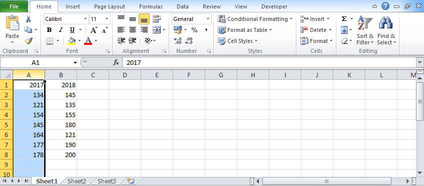
- Let take the Employee Id’s who meet their sales target in the year 2017 in Column 1 whereas Employee Id’s of those candidates who meet their targets in the year 2018 are to be taken in Column 2. Now we have to compare column 1 with column 2.

- Select Column 1 to make it highlight.
- Go to the conditional formatting option available on the home tab.

- By clicking the drop-down list, you will find various conditional formatting options, select New rule.
- You will find various rule types, in which you need to choose “Use a formula to determine which cells to format” option.
- In format values where this formula is the true box, you have to enter formula “=countif($B:$B, $A1).
- Click on the Format button and select the format according to your requirement.

- You can fill color in the cell by clicking on the Fill tab and choose the background color.

- After making this selection, Press on OK button.
- After this, you will get the previous sheet with coloring on the duplicate values.

- Do the same process for Column 2.
This way you can find out the matches by excel compare values in two columns using conditional formatting process.
Excel Compare Two Columns for Differences
To find the different values in two columns, we use conditional formatting and using this formatting we highlight all the differing values.
- We will take the same list as we have taken for the matches. Now we will compare these columns to get the common data and highlighting the different data.
- Choose the columns that you want to compare.
- Click on the conditional formatting and you will find the drop-down menu.

- In this menu, you need to select the Highlight Cell Rules option.
- In its submenu, choose More Rules option and click on it.
- After selecting more rules, you will find another pop up displayed.
- In this pop-up, choose format only unique or duplicate values.
- In Format, all drop-down list, choose unique as an option.
- Then click on format.
- Go to fill tab, and choose a color.
- Press Ok.

- You will find a coloring sheet that is showing unique items.
By following the above method, you can compare two columns in excel to find differences using conditional formatting.
Hence these are the four different ways to compare values and to find the matched and different values. Read all the ways carefully and choose the best way to find the matched and different values using these above formulas. Hope that above formulas to compare two columns with each other were useful.
Related Queries
Q1. How to compare multiple columns in Excel in the same row for matches? Count the total duplicates also.
Ans. We have given the procedure to compare two columns in excel for the same row above. But if you want to compare multiple columns in excel for the same row then see the example
=IF(AND(A2=B2, A2=C2),”Full Match”, “”)
Here we have compared data of column A, column B, and column C. After this, I have applied the above formula in column D and get the result.

Now to count the duplicates, you need to use the Countif function.
=If(CountIf($A2:$E2, $A2)=5, “Full Match”, “”)
Q2. Which operator do you use for matches and differences?
Ans. For matches: =
For differences: <>
Q3. How to compare two different tables and pull matching data?
Ans. For this, you can use Vlookup function or Index & Match formula. To understand this thing in a better way we will take an example. Here we will take two tables and now want to do pull matching data. In the first table, you have a dataset and in the second table, take the list of fruits and then use pull matching data in another column. For pull matching, use the formula
=Index($B$2:$B$6,Match($D2,$A$2:$A$6,0))
Q4. How to remove duplicates in excel?
Ans. To remove duplicate data you need to first find the duplicate values. To find the duplicate, you can use various methods like conditional formatting, Vlookup, If Statement, and many more. To get more details to know the process to remove duplicate values Click Here.
Q5. How to find missing data by comparing two columns in excel?
To understand its concept well, we will take an example here. In this data set, we will put values in column 1 and column 2.
=IsError(VLookup(A2,$B$2:$B$10,1,0))
This formula works where the Vlookup function will check whether the fruit listed in column A is also available in column B or not. IsError will return either True or False.
Q6. I have a database of 100 rows that looks like
A1 Seema
A2 Shanti
A3 Suhasini
A4 Shalini
A5 Shweta
And in another table, you have 50 rows and the data looks like
B1 Shalini
B2 Samir
Now I want to highlight cells available in column A where the data is similar as in column B. Only the matched data gets highlighted and leaving other cells white. I have already tried conditional formatting and it’s not working. Is there any other formula apart from conditional formatting to highlight the matched data?
Ans. There are various options to compare two columns in excel. Here we are going to use Vlookup formula to find whether the value appears in the list or not. For column A, use the formula of Vlookup function:
=Not(ISNA(Vlookup(A1,$B:$B,1,False)))
Drag the corner to other cells. In this formula, the Vlookup will look for the value in Cell A1 comparing it with Column B. The Vlookup function in this formula will return ISNA if the match is not found.
Q7. How to compare two columns that give the result as TRUE when all first columns’ integer values are not less than the second column’s integer values. To solve this problem, I do not require conditional formatting, Vlookup, If Statement, and any other formulas. I need the formula to solve this problem.
Ans. You can use the array formula for solving this problem. The syntax is {=AND(H6:H12>I6:I12)}. This will give you “True” as a result whenever the value of Column H is greater than the value in column I else “False” will be the result.
In this tutorial, we have covered all the Excel functions and formulas. Here we have listed questions that our excel users asked. If you have any other questions then you can mention below in the comment box. We will soon get back with the answer as we receive your question.