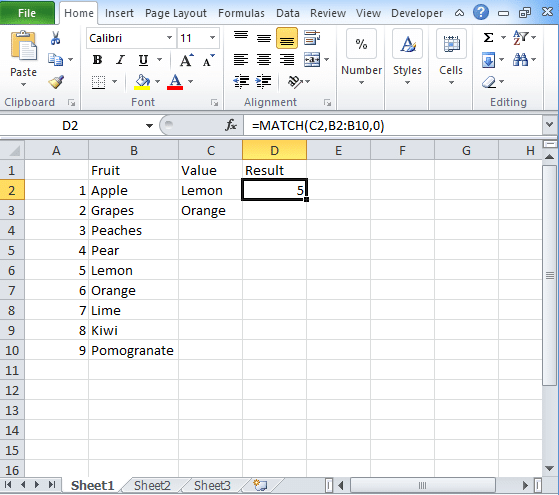
If you want to locate the placement of the lookup value then you need to use Excel Match function. The Match function will offer you an approximate and exact match whereas wildcards are used for partial matches. When you want to retrieve the value of the position which is returned by the MATCH function then you need to use Index function.
Table of Contents
Excel Match Function
We use Excel Match function to get the position of the product in an array. It returns the number that represents the position of the lookup_array. If you use the function with Index then it returns the value of an item. Here you can check the syntax of the Match.
SYNTAX
=MATCH(lookup_value, lookup_array,[Match_type])
Where lookup_value is the value used to match in the lookup_array.
Lookup_array denotes the range of the cells or the array reference.
Match_type is how to match and is denoted by -1, 0, 1 where the default is 1.
Excel Match only returns the position of an item while if you use it with index then you can retrieve the value out of it.
NOTE:
Match_type is 1: It finds the largest value which is less than or equal to the lookup_value and the array is sorted in ascending order.
Match_type is 0: The Match function will return the exact value to the lookup_Value.
Match_type is -1: It finds the smallest value which is greater than or equal to the lookup_value.
Match_type is not present then it is assumed as 1.
Basic Exact Match
If the match type is zero, then the formula gives you an exact match. For example, if you have data in column A and B and you want to find the position. The syntax of this Match function:
D2 = Match(D2,B2:B10,0)
Basic Approximate Match
If match type is 1, then the Match formula will give an approximate match. This will give the largest value which is less than or equal to lookup value.
D2 = Match(D2,B2:B10,1)
Points to remember in using Match Function
- The Match function is not based on case-sensitive.
- It returns the #N/A error if the match will not found.
- In lookup_array, the argument is placed in the descending form True, False,Z….,A….,1, 0, -1, -2…and more.
- If the type of the match is 0 and the value in that parameter is text then you have to use wildcards in the value parameter.
(“*” = Matches the characters sequence and “?” = matches the single character)
Case Sensitive Match Formula
Here you can check the case-sensitive formulas to match the data in excel:
Match (True, Exact(lookup array, lookup value), 0) where,
The exact function compares the lookup value with every element placed in the lookup array. If the cells are equal then it returns either True or False.
Match function compares the TRUE with every value in an array which is an outcome of an Exact. Along with this, it returns the position of the match.
Compare 2 columns (ISNA MATCH)
If you want to perform excel compare two columns for finding out the matches and differences then you need to use the ISNA/MATCH formula. The syntax of the formula is
=If(ISNA(MATCH(1st value in List1, List2,0)), “Not in List 1”, “”)

