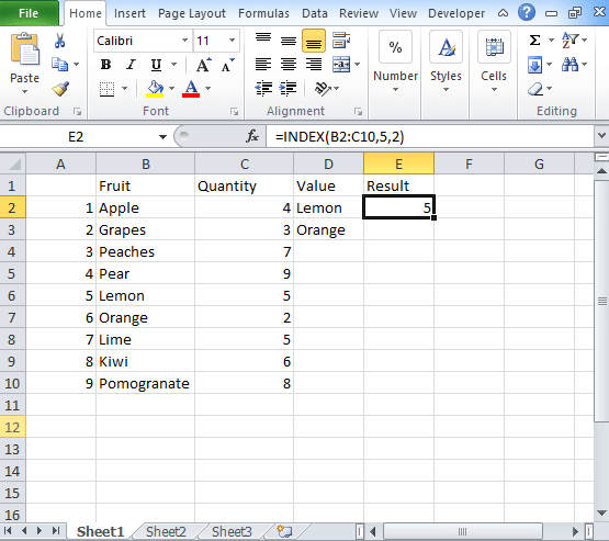
In our previous post, we have already cover Excel Match function. The Match function in excel returns the position of an item in array whereas the Index function in Excel returns the value present in that position in the array. Hence if you want to extract any value from an array then you need to use this index match function excel.
The function will give you the value of an item located at a certain position in an array. You need to use the index function to retrieve the values or complete rows and columns. The excel Index function is used with match function where the Match function is used to find the position of the value and Index function returns the value of the item at that position. The function will return the value present at the given position in the array.
SYNTAX of Index Function
=Index(array, row_num, [col_num], [area_num])
where
Array is the range of cells or constant of an array.
Row_num is the position of the row in an array.
Col_num is the position of the column in the reference or an array.
Area_num is the range in reference that you should use.
For Array format,
In Index Array form, the first thing that comes in the formula is an array. The syntax is
=Index(array, row_num, [col_num])
where
- If you have row_num and col_num then this formula will return the value present in the cell at its intersection.
- If row_num is 0, then this function will return values for the entire row.
- If col_num is 0, then the Index function will return the values of the entire column.
For Reference form,
In this form, the first parameter that comes in syntax is the reference. The reference is supplied to different cell ranges. The syntax of the reference index formula is
=Index(reference, row_num, [col_num], [area_num])
- The function will return the cell reference comes at the intersection between row_num and col_num.
- At the place of reference, you can supply multiple ranges where the area_num indicates the range you use.
How to use Index Function in Excel?
Here you can check the step by step process of using Index function in excel.
- Start with “=Index(“ and choose the area of the table followed by the comma.
- Mention the row number followed by the comma
- Mention the column number followed by the close bracket.
- Get the result.
Excel Index Match Multiple Criteria
By combining the Index and Match function, the formula that comes out is
=Index(range, Match(lookup_value, lookup_range, match_type).
Index Match function works similarly as the vlookup function with only a few changes:
- With index match function, you do not have to count.
- If you are using this function, then you can safely insert the columns.
- If you are using Index Match formula, then you do not have to use two formulas together like Vlookup and hlookup.
The Excel Index Match formula works exactly like vlookup formula. Check the details here and apply the formula to retrieve data. Keep in touch to get more ideas

